In the field of machine learning and particularly in supervised learning, correlation is crucial to predict the target variable with the help of the feature variables. Rarely do we think about causation and the actual effect of a single feature variable or covariate on the target or response. Some even go so far as to say that “correlation trumps causation” like in the book “Big Data: A Revolution That Will Transform How We Live, Work, and Think” by Viktor Mayer-Schönberger and Kenneth Cukier. Following their reasoning, with Big Data there is no need to think about causation anymore, since nonparametric models will do just fine using correlation alone. For many practical use cases, this point of view may seem acceptable — but surely not for all.
Consider for instance you are managing an advertisement campaign with a budget allowing you to send discount vouchers to 10,000 of your customers. Obviously, you want to maximise the outcome of the campaign, meaning you want to focus on customers that buy because they received a voucher. If \(y_{1i}\) and \(y_{0i}\) are the amounts of money spent by a customer \(i\) described by \(x_i\) that either received or did not receive a voucher, we want to find a subset \(I'\subset{}I\) where \(I\) is the set of all former customers with \(|I'|=10,000\) so that \(\sum_{i\in I'}y_{1i} - y_{0i}\) is maximised.
Another example would be to estimate the effect of additional booking options in an online marketplace. A common use case of an online vehicle marketplace is to provide estimations to sellers on the effect that additional booking options (e.g. highlighting, top of page etc.) may have on the selling time of a given vehicle. Likewise, many dealers will be interested in knowing how changing the price of a vehicle will affect the probability of selling the vehicle within a certain period of time or the expected selling time.
These two examples outline the need for methods to estimate the actual causal effect of a controllable covariate onto the response. Before we dip our toes into the deep sea of causal inference, let’s consider a few general aspects. The first and maybe not so obvious point when coming from a supervised learning background is that causal inference is thinking about what did not happen. That means that we don’t know for instance how much a customer that received a voucher would have ordered if they had not received one. This fundamental problem basically renders it an unsupervised learning problem. More interesting aspects of causal inference are summarized in a blog post by Macartan Humphreys on 10 Things to Know About Causal Inference. The question remains how can we estimate the causal effect of a controllable covariate?
Strongly ignorable
The answer to this question lies in another important (and actually the original) use case of causal inference, which is the analysis of therapy effects. In a best-case scenario, the effect of a therapy can be determined in a randomized trial by comparing the response of a treatment group to a control group. In a randomized trial, the allocation of participants to the test or control group is random and thus independent of any covariates \(X\). Following the original paper of Rosenbaum & Rubin 2, in a randomized trial the treatment assignment \(Z\) and the (unobservable) potential outcomes \({Y_1, Y_0}\) are conditionally independent given the covariates \(X\), i.e.
Furthermore, we assume that each participant in the experiment has a chance to receive each treatment, i.e. \(0 < p(Z=1|x) < 1\). The treatment assignment is said to be strongly ignorable if those two conditions hold for our observed covariates \(x\).
Causal effect in a randomized trial
In a randomized trial, the strong ignorability of \(Z\) allows us to estimate the effect of the treatment by comparing the response of the treatment group with that of the control group. The following approach may be used to estimate the individual effect of an additional booking option on a vehicle’s selling time with machine learning methods like a random forest:
- Train the model with the covariates \(X\) and \(Z\) as feature and response \(Y\) as target,
- predict for a given \(x\) the response \(\hat{y}_1\) with \(Z=1\) and \(\hat{y}_0\) with \(Z=0\),
- calculate the effect with \(\hat{y}_1 - \hat{y}_0\) or \(\frac{\hat{y}_1}{\hat{y}_0}\).
In a real-world big-data problem we often have no control over the experimental setup — we are just left with the data. This happens for instance in observational studies. Imagine for instance the treatment with an experimental drug having strong side-effects that might cure a life-threatening disease. A controlled, randomized experiment where the control groups gets a placebo might be impracticable or even unethical.
In such a nonrandomized experiment, there is no proper mathematical way to check if the treatment is strongly ignorable3. According to Pearl4 by now assuming strong ignorability we are basically assuming that our covariate set \(X\) is admissible, i.e. \(p(y|\mathrm{do}(z))=\sum_{x}p(y|x,z)p(x)\). Here, Pearl’s \(\mathrm{do}\)-notation \(p(y|\mathrm{do}(z))\) denotes the “causal effect” of \(Z\) on \(Y\), i.e. the distribution of \(Y\) after setting variable \(Z\) to a constant \(Z = z\) by external intervention. In practice, the assumption of admissibility of \(X\) is often used to estimate a causal effect. This led to incorrect results in some studies as well as controversies3, so one should always be aware that the entire causal analysis depends on the validity of this assumption.
So far, we have not only assumed admissibility of \(X\) but also a randomized trial for our approach. Therefore, we should check beforehand that \(X ⫫ Z\), (which is a necessary but not sufficient condition), before applying the aforementioned approach. This can be verified by using \(X\) to predict \(Z\). If this is not possible, and thus \(p(z|x) = p(z)\), the former approach is viable. But what if \(Z\) is not independent of \(X\) — as is often the case with real-world data. For instance, dealers of expensive vehicle brands might be more willing to spend money and therefore tend to use more booking options. The data from the last marketing campaign presumingly includes a bias induced by the current strategy of the marketing department on how to pick customers that get a voucher. In these cases, we have to isolate the effect of \(Z\) from our covariates \(X\).
Propensity score
By predicting \(Z\) based on \(X\), we have estimated the propensity score, i.e. \(p(Z=1|x)\). This of course assumes that we have used a classification method that returns probabilities for the classes \(Z=1\) and \(Z=0\). Let \(e_i=p(Z=1|x_i)\) be the propensity score of the \(i\)-th observation, i.e. the propensity of the \(i\)-th participant getting the treatment (\(Z=1\)).
We can use the propensity score to define weights \(w_i\) to create a synthetic sample in which the distribution of measured baseline covariates is independent of treatment assignment5, i.e.
where \(z_i\) indicates if the \(i\)-th subject was treated.
The covariates from our data sample \(x_i\) are then weighted by \(w_i\) to eliminate the correlation between \(X\) and \(Z\), which is a technique known as inverse probability of treatment weighting (IPTW). This allows us to estimate the causal effect via the following approach:
- Train a model with covariates \(X\) to predict \(Z\),
- calculate the propensity scores \(e_i\) by applying the trained model to all \(x_i\),
- train a second model with covariates \(X\) and \(Z\) as features and response \(Y\) as target by using \(w_i\) as sample weight for the \(i\)-th observation,
- use this model to predict the causal effect like in the randomized trial approach.
IPTW is based on a simple intuition. For a randomized trial with \(p(Z=1)=k\) the propensity score would be equal for all patients, i.e. \(e_i=\frac{1}{k}\) and thus \(w_i=k\). In a nonrandomized trial, we would assign low weights to samples where the assignment of treatment matches our expectation and high weights otherwise. By doing so, we draw the attention of the machine learning algorithm to the observations where the effect of treatment is most prevalent, i.e. least confounded with the covariates.
Python implementation
We can set up a synthetic experiment to demonstrate and evaluate this method with the help of Python and Scikit-Learn. A synthetic experiment is appropriate to address the fundamental problem of causal inference described above. With real data, we don’t know what would have happened if we had not treated someone, sent a voucher or not booked that additional option and vice versa. Therefore, we derive a model that describes the relationship of \(X\) to \(Y\) as well as the effect of \(Z\) on \(Y\). We use this model to generate observational data where for each sample \(x_i\) we either have \(Z=1\) or \(Z=0\) and thus incomplete information in our data. Our task is now to estimate the effect of \(Z\) with the help of the generated data.
The following portion of this article is available for download as a Jupyter notebook.
from math import exp, log

import numpy as np
import pandas as pd
import scipy as sp
from scipy import stats
from scipy.special import expit

from sklearn.ensemble import RandomForestClassifier, RandomForestRegressor
from sklearn.linear_model import LogisticRegression
from sklearn.naive_bayes import GaussianNB
from sklearn.calibration import CalibratedClassifierCV

import statsmodels.api as sm
import statsmodels.formula.api as smf
import matplotlib.pyplot as plt

%matplotlib inline

import seaborn as sns
sns.set_style("whitegrid")
sns.set_context("notebook", font_scale=1.5, rc={"lines.linewidth": 2.5})
plt.rcParams['figure.figsize'] = 10, 8

np.seterr(divide='ignore', invalid='ignore')
np.random.seed(42)
Model
Assume we have patients characterized by sex and age suffering from some disease with different severities. The recovery time of a patient depends only on the sex, age, severity and if the patient is on medication. Let the expected recovery time in days \(t_{recovery}\) be defined as
where \(I\) is an indicator function. Furthermore, we will assume a Poisson distribution in order to generate some synthetic data of our patient’s recovery time. Due to our definition, treating the disease with medication reduces the recovery time to \(\exp(-1)\approx 0.37\) of the recovery time having no treatment. Although the recovery time is specific to each patients, i.e. his/her features, the effect of a reduction to 37% of the recovery time without medication is the same for all patients.
def exp_recovery_time(sex, age, severity, medication):
    return exp(2+0.5*sex+0.03*age+2*severity-1*medication)

def rvs_recovery_time(sex, age, severity, medication, *args):
    return stats.poisson.rvs(exp_recovery_time(sex, age, severity, medication))
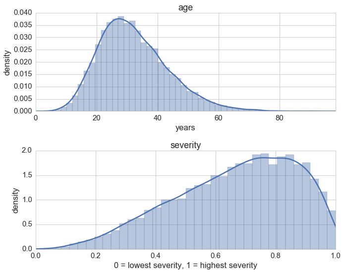
For the features of the patients we will use a Beta distribution to show how badly the disease struck the patients, a Gamma distribution for the age of our patients and a Bernoulli distribution for the gender of the patients.
N = 10000  # number of observations, i.e. patients
sexes = np.random.randint(0, 2, size=N)  # sex == 1 if male otherwise female
ages_dist = stats.gamma(8, scale=4)
ages = ages_dist.rvs(size=N)
sev_dist = stats.beta(3, 1.5)
severties = sev_dist.rvs(size=N)
It’s always a good idea to take a look at the nontrivial distributions:
f, (ax1, ax2) = plt.subplots(2)
ax1.set_title('age')
ax1.set_xlabel('years')
ax1.set_ylabel('density')
ax1.set_xlim(0, np.max(ages))
ax2.set_title('severity')
ax2.set_xlabel('0 = lowest severity, 1 = highest severity')
ax2.set_ylabel('density')
ax2.set_xlim(0, 1)
sns.distplot(ages, ax=ax1)
sns.distplot(severties, ax=ax2)
plt.tight_layout();
Randomized trial
In a controlled randomized trial we randomly select patients and assign them with a chance of 50% to either treatment or control. Therefore, the assignment of treatement is completely random and independent.
meds = np.random.randint(0, 2, size=N)
We assemble everything in a dataframe also including a constant column.
const = np.ones(N)
df_rnd = pd.DataFrame(dict(sex=sexes, age=ages, severity=severties, medication=meds, const=const))
features = ['sex', 'age', 'severity', 'medication', 'const']
df_rnd = df_rnd[features] # to enforce column order
df_rnd['recovery'] = df_rnd.apply(lambda x: rvs_recovery_time(*x) , axis=1)
df_rnd.head()
| sex | age | severity | medication | const | recovery | |
|---|---|---|---|---|---|---|
| 0 | 0 | 24.5187 | 0.85895 | 1 | 1 | 34 |
| 1 | 1 | 11.0802 | 0.905123 | 0 | 1 | 97 |
| 2 | 0 | 37.0149 | 0.601475 | 0 | 1 | 77 |
| 3 | 0 | 35.6577 | 0.74984 | 1 | 1 | 39 |
| 4 | 0 | 36.7352 | 0.38546 | 1 | 1 | 18 |
df_rnd.describe()
| sex | age | severity | medication | const | recovery | |
|---|---|---|---|---|---|---|
| count | 10000 | 10000 | 10000 | 10000 | 10000 | 10000 |
| mean | 0.498700 | 32.160968 | 0.666299 | 0.497400 | 1 | 76.085700 |
| std | 0.500023 | 11.243333 | 0.20101 | 0.500018 | 0 | 63.304659 |
| min | 0.000000 | 4.508904 | 0.0298182 | 0.000000 | 1 | 0.000000 |
| 25% | 0.000000 | 24.044093 | 0.525905 | 0.000000 | 1 | 33.000000 |
| 50% | 0.000000 | 30.760101 | 0.693532 | 0.000000 | 1 | 57.000000 |
| 75% | 1.000000 | 38.922208 | 0.829290 | 1.000000 | 1 | 99.000000 |
| max | 1.000000 | 98.330906 | 0.999327 | 1.000000 | 1 | 805.000000 |
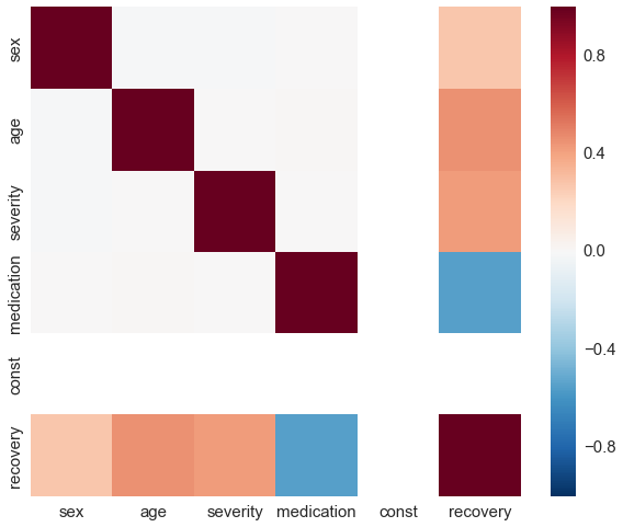
By construction, there is no correlation between medication and any other covariate.
sns.heatmap(df_rnd.corr(), vmin=-1, vmax=1);
To get started we use a Poisson regression to estimate the coefficients of our formula for \(\mathbf{E}(t_{recovery})\) from the generated data. Of course we expect to see approximately the same coefficients since Poisson regression assumes the exact same model that generated our data.
glm = sm.GLM(df_rnd['recovery'], df_rnd[features], family=sm.families.Poisson())
res = glm.fit()
res.summary()
| Dep. Variable: | recovery | No. Observations: | 10000 |
|---|---|---|---|
| Model: | GLM | Df Residuals: | 9995 |
| Model Family: | Poisson | Df Model: | 4 |
| Link Function: | log | Scale: | 1.0 |
| Method: | IRLS | Log-Likelihood: | -34429. |
| Date: | Sat, 15 Apr 2017 | Deviance: | 10080. |
| Time: | 20:13:45 | Pearson chi2: | 1.00e+04 |
| No. Iterations: | 5 |
| coef | std err | z | P>|z| | [0.025 | 0.975] | |
|---|---|---|---|---|---|---|
| sex | 0.4994 | 0.002 | 211.934 | 0.000 | 0.495 | 0.504 |
| age | 0.0301 | 8.95e-05 | 335.807 | 0.000 | 0.030 | 0.030 |
| severity | 2.0000 | 0.006 | 309.610 | 0.000 | 1.987 | 2.013 |
| medication | -1.0024 | 0.003 | -387.721 | 0.000 | -1.007 | -0.997 |
| const | 1.9990 | 0.006 | 326.234 | 0.000 | 1.987 | 2.011 |
Now we use a randome forest which is a pretty standard machine learning method to estimate the individual effects of the treatment on the patients. We fit the model and predict for each patient the recovery time assuming medication, i.e. medication column is 1, as well as assuming no medication, i.e. medication column is 0. Subsequently we divide the prediction assuming medication by the prediction assuming no medication to get an estimation of the treatment’s effect.
reg = RandomForestRegressor()
X = df_rnd[features].as_matrix()
y = df_rnd['recovery'].values
reg.fit(X, y)
X_neg = np.copy(X)
# set the medication column to 0
X_neg[:, df_rnd.columns.get_loc('medication')] = 0
X_pos = np.copy(X)
# set the medication column to 1
X_pos[:, df_rnd.columns.get_loc('medication')] = 1

preds_rnd = reg.predict(X_pos) / reg.predict(X_neg)
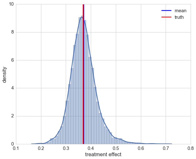
Let’s take a look at the distribution of individual effects. Even though we are assuming no model by using a random forest, our estimations of the treatment effect look decent.
ax = sns.distplot(preds_rnd)
ax.set_xlabel('treatment effect')
ax.set_ylabel('density')
plt.axvline(np.mean(preds_rnd), label='mean')
plt.axvline(np.exp(-1), color='r', label='truth')
plt.legend();
Nonrandomized trial
To make things a bit more interesting, we put now patients on a treatment depending on their sex and severity of the illness. Since men often suffer more than women from the same illness, e.g. man flu, they tend to complain more and thus are more likely to convince the doctor of prescibing a medication. Thereafter we generate the recovery time again and follow the same procedure as before in the randomized trial.
def get_medication(sex, age, severity, medication, *args):
    return int(1/3*sex + 2/3*severity + 0.15*np.random.randn() > 0.8)

df_obs = df_rnd.copy().drop('recovery', axis=1)
df_obs['medication'] = df_obs.apply(lambda x: get_medication(*x), axis=1)
df_obs['recovery'] = df_obs.apply(lambda x: rvs_recovery_time(*x), axis=1)
df_obs.describe()
| sex | age | severity | medication | const | recovery | |
|---|---|---|---|---|---|---|
| count | 10000.000000 | 10000.000000 | 10000.000000 | 10000.000000 | 10000.0 | 10000.000000 |
| mean | 0.498700 | 32.160968 | 0.666299 | 0.251900 | 1.0 | 85.029100 |
| std | 0.500023 | 11.243333 | 0.201010 | 0.434126 | 0.0 | 51.400825 |
| min | 0.000000 | 4.508904 | 0.029818 | 0.000000 | 1.0 | 8.000000 |
| 25% | 0.000000 | 24.044093 | 0.525905 | 0.000000 | 1.0 | 50.000000 |
| 50% | 0.000000 | 30.760101 | 0.693532 | 0.000000 | 1.0 | 73.000000 |
| 75% | 1.000000 | 38.922208 | 0.829290 | 1.000000 | 1.0 | 106.000000 |
| max | 1.000000 | 98.330906 | 0.999327 | 1.000000 | 1.0 | 624.000000 |
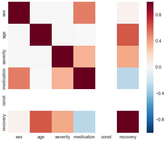
sns.heatmap(df_obs.corr(), vmin=-1, vmax=1);
glm = sm.GLM(df_obs['recovery'], df_obs[features], family=sm.families.Poisson())
res = glm.fit()
res.summary()
| Dep. Variable: | recovery | No. Observations: | 10000 |
|---|---|---|---|
| Model: | GLM | Df Residuals: | 9995 |
| Model Family: | Poisson | Df Model: | 4 |
| Link Function: | log | Scale: | 1.0 |
| Method: | IRLS | Log-Likelihood: | -35645. |
| Date: | Sat, 15 Apr 2017 | Deviance: | 10018. |
| Time: | 20:13:47 | Pearson chi2: | 9.98e+03 |
| No. Iterations: | 5 |
| coef | std err | z | P>|z| | [0.025 | 0.975] | |
|---|---|---|---|---|---|---|
| sex | 0.5043 | 0.002 | 203.256 | 0.000 | 0.499 | 0.509 |
| age | 0.0299 | 8.58e-05 | 349.024 | 0.000 | 0.030 | 0.030 |
| severity | 1.9996 | 0.006 | 313.055 | 0.000 | 1.987 | 2.012 |
| medication | -1.0063 | 0.003 | -302.201 | 0.000 | -1.013 | -1.000 |
| const | 2.0013 | 0.006 | 340.305 | 0.000 | 1.990 | 2.013 |
The first stunning result is that the Poisson regression is still able to correctly estimate the coefficients of our model. This is due to the model dependence and in realistic cases actually a bad thing. In a nutshell, model dependence means that the inference of the causal effect depends on the chosen model. In our case, the assumptions about the relation of the covariates in the Poisson regression extrapolates our data and thus makes our results heavily depend on the Poisson model. Since we also used a Poisson model to generate the data we are lucky but this is in reality rarely the case. Let’s check how the random forest performs.
reg = RandomForestRegressor()
X = df_obs[features].as_matrix()
y = df_obs['recovery'].values
reg.fit(X, y)
X_neg = np.copy(X)
X_neg[:, df_obs.columns.get_loc('medication')] = 0
X_pos = np.copy(X)
X_pos[:, df_obs.columns.get_loc('medication')] = 1

preds_no_rnd = reg.predict(X_pos) / reg.predict(X_neg)

ax = sns.distplot(preds_no_rnd)
ax.set_xlabel('treatment effect')
ax.set_ylabel('density')
plt.axvline(np.mean(preds_no_rnd), label='mean')
plt.axvline(np.exp(-1), color='r', label='truth')
plt.legend();
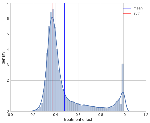
The distribution is now quite skewed and we can see that for a lot of our patients their individual treatment effect is heavily underestimated. This due to the fact that the random forest overrates the impact of a patient’s sex which is highly correlated with the medication.
Inverse probability of treatment weighting
To deminish the impact of other covariates onto the effect of medication we will no calculate the propensity score and use inverse probability of treatment weighting (IPTW). In order to do that we use a classification to predict the probability of a patient to be treated. This can be accomplished by Scikit-Learn’s predict_proba method that is available for most classificators. Don’t be fooled by the name though, in most cases (logistic regression is an exception) the probabilites are not calibrated and cannot be relied on. To fix this, we use the CalibratedClassifierCV in order to get proper probabilities (and it doesn’t hurt applying it for logistic regression too). After that we calculate the inverse probability of treatment weights and pass those as sample weights to the estimator during the fit.
# classifier to estimate the propensity score
cls = LogisticRegression(random_state=42)
#cls = GaussianNB()  # another possible propensity score estimator

# calibration of the classifier
cls = CalibratedClassifierCV(cls)

X = df_obs[features].drop(['medication'], axis=1).as_matrix()
y = df_obs['medication'].values
cls.fit(X, y)
propensity = pd.DataFrame(cls.predict_proba(X))
propensity.head()
| 0 | 1 | |
|---|---|---|
| 0 | 0.947430 | 0.052570 |
| 1 | 0.170632 | 0.829368 |
| 2 | 0.992034 | 0.007966 |
| 3 | 0.975970 | 0.024030 |
| 4 | 0.998434 | 0.001566 |
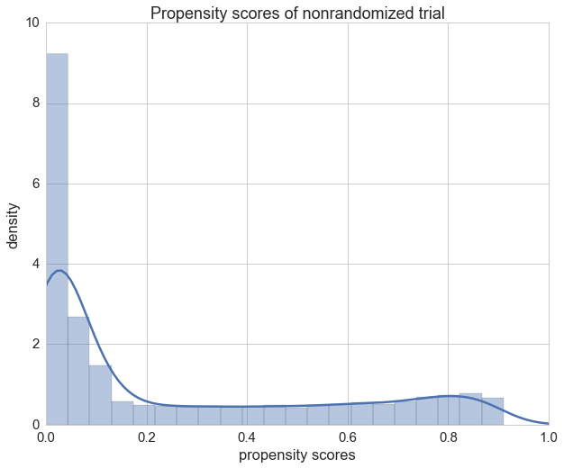
We can see that the propensity scores of our patients in the randomized trial vary a lot as expected.
ax = sns.distplot(propensity[1].values)
ax.set_xlim(0, 1)
ax.set_title("Propensity scores of nonrandomized trial")
ax.set_xlabel("propensity scores")
ax.set_ylabel('density');
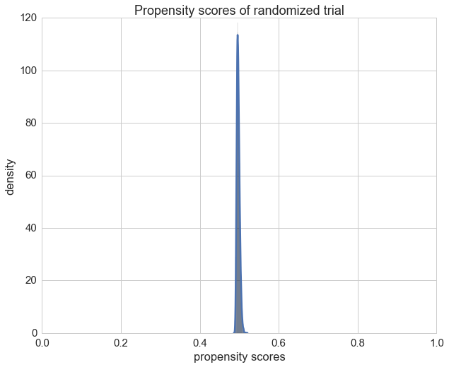
Only for comparison we can also plot the propensity scores of the randomized trail and check if the propensity score is \(\frac{1}{2}\) as expected.
X = df_rnd[features].drop(['medication'], axis=1).as_matrix()
y = df_rnd['medication'].values
cls.fit(X, y)
ax = sns.distplot(cls.predict_proba(X)[:,1]);
ax.set_xlim(0, 1)
ax.set_title("Propensity scores of randomized trial")
ax.set_xlabel("propensity scores")
ax.set_ylabel('density');
We now calculate at this point the inverse probability of treatment weights (IPTWs) with the help of the propensity scores of the nonrandomized trial.
# DataFrame's lookup method extracts the column index
# provided by df2['medication'] for each row
df_obs['iptw'] = 1. / propensity.lookup(
   np.arange(propensity.shape[0]), df_obs['medication'])

df_obs.describe()
| sex | age | severity | medication | const | recovery | iptw | |
|---|---|---|---|---|---|---|---|
| count | 10000 | 10000 | 10000 | 10000 | 10000 | 10000 | 10000 |
| mean | 0.498700 | 32.160968 | 0.666299 | 0.251900 | 1.0 | 85.029100 | 1.860499 |
| std | 0.500023 | 11.243333 | 0.201010 | 0.434126 | 0.0 | 51.400825 | 4.455724 |
| min | 0.000000 | 4.508904 | 0.029818 | 0.000000 | 1.0 | 8.000000 | 1.000105 |
| 25% | 0.000000 | 24.044093 | 0.525905 | 0.000000 | 1.0 | 50.000000 | 1.016131 |
| 50% | 0.000000 | 30.760101 | 0.693532 | 0.000000 | 1.0 | 73.000000 | 1.093217 |
| 75% | 1.000000 | 38.922208 | 0.829290 | 1.000000 | 1.0 | 106.000000 | 1.449351 |
| max | 1.000000 | 98.330906 | 0.999327 | 1.000000 | 1.000000 | 624.000000 | 184.561863 |
The poisson regression benefits from using the IPTWs as weights since the Z-scores of the coefficients increase.
glm = sm.GLM(df_obs['recovery'], df_obs[features],
             family=sm.families.Poisson(),
             freq_weights=df_obs['iptw'])
res = glm.fit()
res.summary()
| Dep. Variable: | recovery | No. Observations: | 10000 |
|---|---|---|---|
| Model: | GLM | Df Residuals: | 18599 |
| Model Family: | Poisson | Df Model: | 4 |
| Link Function: | log | Scale: | 1.0 |
| Method: | IRLS | Log-Likelihood: | -64795. |
| Date: | Sat, 15 Apr 2017 | Deviance: | 18482. |
| Time: | 20:13:49 | Pearson chi2: | 1.83e+04 |
| No. Iterations: | 5 |
| coef | std err | z | P>|z| | [0.025 | 0.975] | |
|---|---|---|---|---|---|---|
| sex | 0.5018 | 0.002 | 294.822 | 0.000 | 0.498 | 0.505 |
| age | 0.0298 | 6.56e-05 | 454.701 | 0.000 | 0.030 | 0.030 |
| severity | 2.0016 | 0.005 | 429.319 | 0.000 | 1.992 | 2.011 |
| medication | -1.0017 | 0.002 | -534.776 | 0.000 | -1.005 | -0.998 |
| const | 2.0055 | 0.005 | 441.204 | 0.000 | 1.997 | 2.014 |
Let’s check how our random forest does with the help of IPTWs.
reg = RandomForestRegressor(random_state=42)
X = df_obs[features].as_matrix()
y = df_obs['recovery'].values
reg.fit(X, y, sample_weight=df_obs['iptw'].values)
X_neg = np.copy(X)
X_neg[:, df_obs.columns.get_loc('medication')] = 0
X_pos = np.copy(X)
X_pos[:, df_obs.columns.get_loc('medication')] = 1

preds_propensity = reg.predict(X_pos) / reg.predict(X_neg)

ax = sns.distplot(preds_propensity)
ax.set_xlabel('treatment effect')
ax.set_ylabel('density')
plt.axvline(np.mean(preds_propensity), label='mean')
plt.axvline(np.exp(-1), color='r', label='truth')
plt.legend();
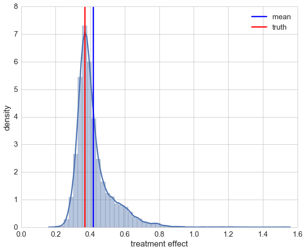
After taking a brief look at the distribution we see that using IPTW drastically improved the estimation of the treatment’s causal effect. On second glance though, it can also be seen that for a few samples we have over-estimation beyond 1. Looking at those patients it can be seen that all of them are female. This indicates that the causal effect for these cases could not be captured maybe due to the bagging approach in random forests. For most of the patients the estimation of the causal effect is improved though.
A direct comparison is given below, showing the estimations of treatment effects for the randomized trail, the non-randomized trail and the non-randomized with IPTW application.
sns.distplot(preds_rnd, label='randomized')
sns.distplot(preds_no_rnd, label='non-randomized')
ax = sns.distplot(preds_propensity, label='non-randomized with IPTW')
ax.set_xlabel('treatment effect')
ax.set_ylabel('density')
plt.legend();
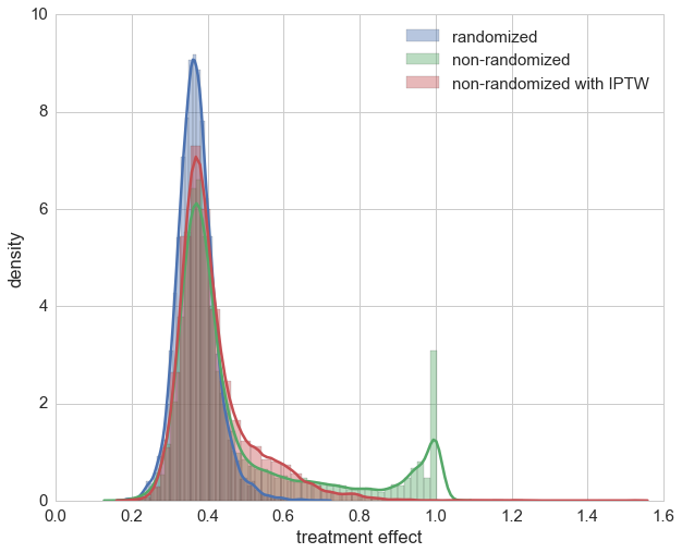
The actual trick of IPTW is that sample weights are chosen in such a way that the correlation of other covariates and the medication is decreased. With the help of a weighted correlation this can also be illustrated. Remarkably enough, neither Numpy, Scipy, Pandas nor StatsModels seem to directly provide a weigthed correlation function, only weighted covariance, which we use to define a weighted correlation.
def weighted_corr(m, w=None):
    if w is None:
        w = np.ones(m.shape[0])
    cov = np.cov(m, rowvar=False, aweights=w, ddof=0)
    sigma = np.sqrt(np.diag(cov))
    return cov / np.outer(sigma, sigma)
Here is the original correlation of the nonrandomized trial again by setting all weights to 1.
sel_cols = [col for col in df_obs.columns if col != 'iptw']
orig_corr = weighted_corr(df_obs[sel_cols].as_matrix(), w=np.ones(df_obs.shape[0]))
orig_corr = pd.DataFrame(orig_corr, index=sel_cols, columns=sel_cols)
orig_corr
| sex | age | severity | medication | const | recovery | |
|---|---|---|---|---|---|---|
| sex | 1.000000 | -0.013332 | -0.012855 | 0.509914 | NaN | 0.046250 |
| age | -0.013332 | 1.000000 | 0.005086 | -0.002818 | NaN | 0.622472 |
| severity | -0.012855 | 0.005086 | 1.000000 | 0.348317 | NaN | 0.378225 |
| medication | 0.509914 | -0.002818 | 0.348317 | 1.000000 | NaN | -0.276164 |
| const | NaN | NaN | NaN | NaN | NaN | NaN |
| recovery | 0.046250 | 0.622472 | 0.378225 | -0.276164 | NaN | 1.000000 |
sns.heatmap(orig_corr, vmin=-1, vmax=1);
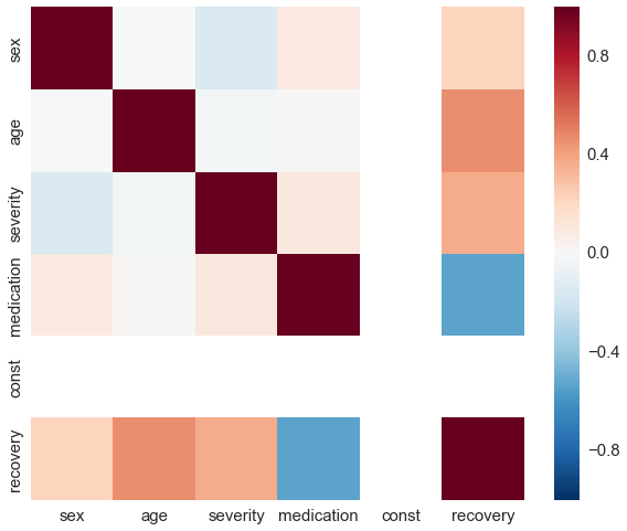
Using the IPTWs the correlation reduces quite a bit.
iptw_corr = weighted_corr(df_obs[sel_cols].as_matrix(), w=df_obs['iptw'].values)
iptw_corr = pd.DataFrame(iptw_corr, index=sel_cols, columns=sel_cols)
iptw_corr
| sex | age | severity | medication | const | recovery | |
|---|---|---|---|---|---|---|
| sex | 1.000000 | -0.001601 | -0.154496 | 0.087948 | NaN | 0.222515 |
| age | -0.001601 | 1.000000 | -0.028975 | 0.014248 | NaN | 0.461467 |
| severity | -0.154496 | -0.028975 | 1.000000 | 0.103541 | NaN | 0.369249 |
| medication | 0.087948 | 0.014248 | 0.103541 | 1.000000 | NaN | -0.531669 |
| const | NaN | NaN | NaN | NaN | NaN | NaN |
| recovery | 0.222515 | 0.461467 | 0.369249 | -0.531669 | NaN | 1.000000 |
sns.heatmap(iptw_corr, vmin=-1, vmax=1);
Final notes
“With great power comes great responsibility” so they say, and IPTW is surely a weapon of math destruction that needs to be handled carefully. Keep in mind that a controlled randomized experiment remains the gold standard by which to estimate a causal effect and should always be preferred. But when reality hits us hard and we have just the data, i.e. no influence on the experiment generating it, we saw that IPTW improves causal inference to some extent.
Furthermore, the demonstrated technique relies on several things. First, \(X\) needs to be admissible — which cannot be practically checked. But we can investigate how the treatment was assigned in our data. In our campaign example, that would mean asking the marketing department about their former strategy when sending vouchers to customers. Then we could verify that the data includes all factors on which their strategy relied. Second, we need an accurate method of estimating the propensity scores for this approach to work. For the sake of simplicity, our demonstration did not check the prediction quality of our machine learning models on a test set, which would be advisable in a real application. The application of machine learning models should always encompass training, validation, test splits and a proper cost functional.
That said, propensity score techniques like IPTW can be very useful. Results can be improved further by first using only the covariates to estimate the recovery time, followed by a residual training with the treatment and the sample weighting to further guide the machine learning algorithm by isolating the causal effect of the treatment — but this is beyond the scope of this post. An overview of other propensity score methods like propensity score matching, stratification on the propensity score and covariate adjustment using the propensity score are well explained in the propensity score methods introduction by Peter Austin5.
PyData meetup talk
A talk about this blog post was presented at PyData meetup in Berlin, April 19th:
References
-
E. Stuart; The why, when, and how of propensity score methods for estimating causal effects; Johns Hopkins Bloomberg School of Public Health, 2011 ↩
-
Paul R. Rosenbaum, Donald B. Rubin; “The Central Role of the Propensity Score in Observational Studies for Causal Effects”; Biometrika, Vol. 70, No. 1., Apr., 1983, pp. 41-55 ↩
-
Judea Pearl; “CAUSALITY - Models, Reasoning and Inference”; 2nd Edition, 2009, pp. 348-352 ↩↩
-
Judea Pearl; “CAUSALITY - Models, Reasoning and Inference”; 2nd Edition, 2009, pp. 341-344 ↩
-
Peter C. Austin; “An Introduction to Propensity Score Methods for Reducing the Effects of Confounding in Observational Studies”; Multivariate Behav Res. 2011 May; 46(3): pp. 399–424 ↩↩
Comments
comments powered by Disqus